
| |
Manual |
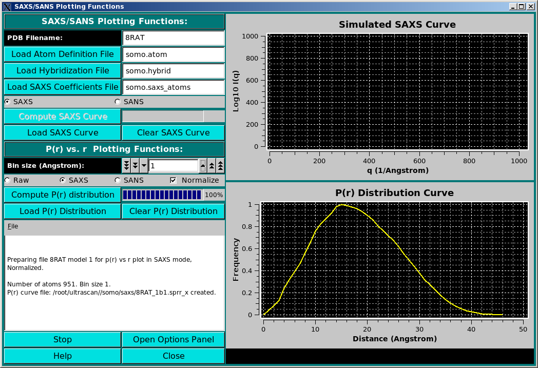
Small-Angle X-ray or Neutron Scattering (SAXS or SANS) I(q) vs. q curves, and pair-distance distribution curves P(r) vs. r, can be generated by this new module from either a PDB file or a bead model. As of January, 2010, only the P(r) vs. r function is active, and is described below.
The P(r) vs. r function can be computed in either "Raw", "SAXS", or "SANS" modes, as selected using the checboxes provided. The equation used is:
P(r) = &Sigmai &Sigmaj [(bi * bj / < b >2) * &delta(r - rij)]
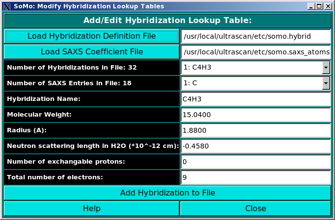
where the bi and bj are: 1- set to "1" for the "Raw" computations; 2- are the number of electrons of the i and j atomic groups for the SAXS computations; and 3- are the neutron scattering lengths of the i and j atomic groups at the set D2O fraction Y for the SANS computations. The Kronecker's delta &delta(r - rij) is applied to the distances rij between the atom's i and j centers for every bin r. The resolution is controlled by the Bin size (Angstroms): field (default: 1 A). For calculations carried on the original PDB structure, the number of electrons are tabulated in the hybridization table). For bead models, only the Raw option is currently (March 2010) active. In a future release, when generating a bead model the number of electrons of the atoms "assigned" to the bead will be summed up and written in the bead model file (9th column), and could then be used in the P(r) vs. r computations. Similarly, for the SANS computations directly on a PDB structure, the neutron scattering lengths are computed at the set D2O fraction Y (b(Y)i and b(Y)j, computed as explained here), and the only the Raw option is currently (March 2010) active for bead models. In a future release, when generating a bead model the b(0) values and the number of exchangeable H of the atoms "assigned" to each bead will be summed up and written in the bead model file as the 10th and 11th columns, respectively. The computation of the b(Y)i and b(Y)j at the set D2O fraction Y could then be carried out for the evaluation of the SANS P(r) vs. r distribution for a bead model.
By pressing the Compute P(r) distribution button a 3-columns file is created, containing the r, the non-normalized P(r), and the normalized P(r) values, respectively. The Normalize clickbox will affect which kind is then shown in the graphic window on the right side, which will automatically rescale upon adding a new graph. The files will be saved in the /somo/SAXS/ directory and will have the extension sprr_r for the "Raw" setting, .sprr_x for the SAXS setting, and .sprr_n for the SANS setting. In addition, a suffix containing the bin size used (e.g., b1 for bin size = 1) will be added at the end of the PDB or bead model filename. For the SANS-type files, a suffix recalling the the D2O fraction will be also added (e.g., D05 for D2O fraction = 0.5). If a file with the same filename already exist, a prompt will appear asking if it should be overwritten or not. In the latter case, the P(r) vs. r distribution will be computed and shown in the graphic window, but not saved to a new file. The graphic window will show every new P(r) vs. r curve in a different color, without erasing curves already present (we plan to add a side bar with a correspondence between the colors and the files). A previously-generated, or experimentally-derived P(r) vs. r curve can be uploaded in the graphic window by pressing the Load P(r) Distribution button, and the graphic window can be cleared by pressing the Clear P(r) Distribution button. Progress in the operations is reported in the advancement bar on the side of the Compute P(r) distribution button, and in the text window below the buttons. Stop will halt the current operation, and the option panel containing the settings controlling the operations, such as the D2O fraction (see here), can be directly accessed by pressing the Open Options Panel button.
This document is part of the UltraScan Software Documentation
distribution.
Copyright © notice.
The latest version of this document can always be found at:
http://www.ultrascan.uthscsa.edu
Last modified on February 26, 2010